Click here to access Github repo containing relevant code or continue reading below on for non-technical description of the project.
Technologies/Skills Used
- Convolutional Neural Network (CNN)
- PyTorch
- PyTorch Lightning
- Albumentations
- Azure Cloud Compute via Microsoft Planetary Computer
- Weights and Biases
Problem Description
According to NASA, only about 30% of the Earth’s land is completely free of clouds. This cloud cover presents a major challenge for satellite imagery analysis since clouds often obscure the land features we want to see. Such a hindrance can impede any number of tasks, from monitoring deforestation to estimating energy consumption. The goal of the project is to create an algorithm that can identify which pixels in a 512x512 pixel image are clouds and which are not clouds. For the uninitiated, the project involves semantic segmentation, or the assignment of individual pixels from an image to particular groups. I completed this project alongside two graduate student classmates as part of the Applied Machine Learning course from UC Berkeley’s Master’s of Information and Data Science program.
The link to our Github repo for this particular project can be found here.
Data
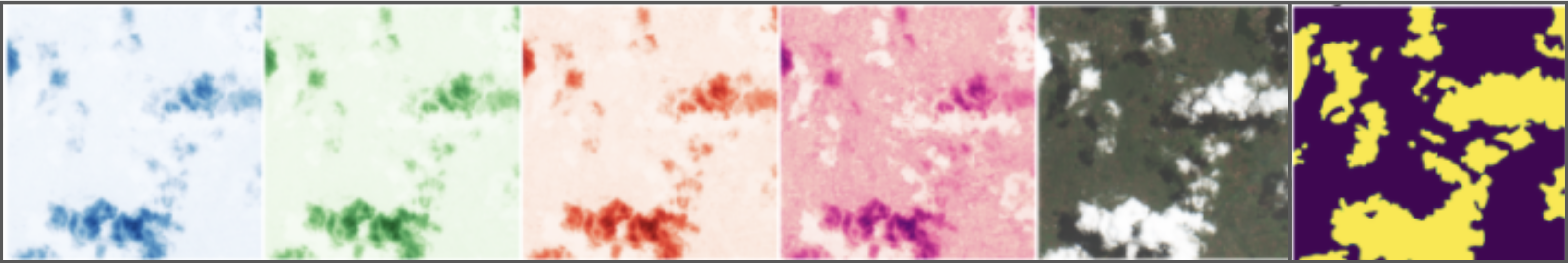
Microsoft’s Planetary Computer stores 10,986 “chips” from the European Space Agency’s Sentinel 2 satellites, comprising roughly 28 GB of data in total. Every chip contains multiple images, each capturing a certain bandwidth of light, for instance from the blue, green, red, and near infrared spectrums. These different bands can be combined to create a human-readable image. Additionally, each chip also came with a mask highlighting which pixels were cloud pixels and where were not.
Solution
To identify clouds, we used PyTorch and its associated PyTorch Lightning library to create convolution neural network running in Microsoft’s Planetary Computer. A basic convolutional neural network using a U-Net archiecture and a ResNet34 pretrained backbone achieved a baseline Intersection over Union (IoU) score of 0.887 on the validation set, where IoU is the conventional performance metric for semantic segmentation.
To improve upon this baseline, we first cleaned the data, manually removing 762 chips with mislabeled masks. From there, we split the data into training, validation, and test sets and then conducted a series of experiments to find out which backbones, optimizers, schedulers, cost functions, and augmentations resulted in superior performance. The execution of each model was captured by Weights and Biases, as shown below.
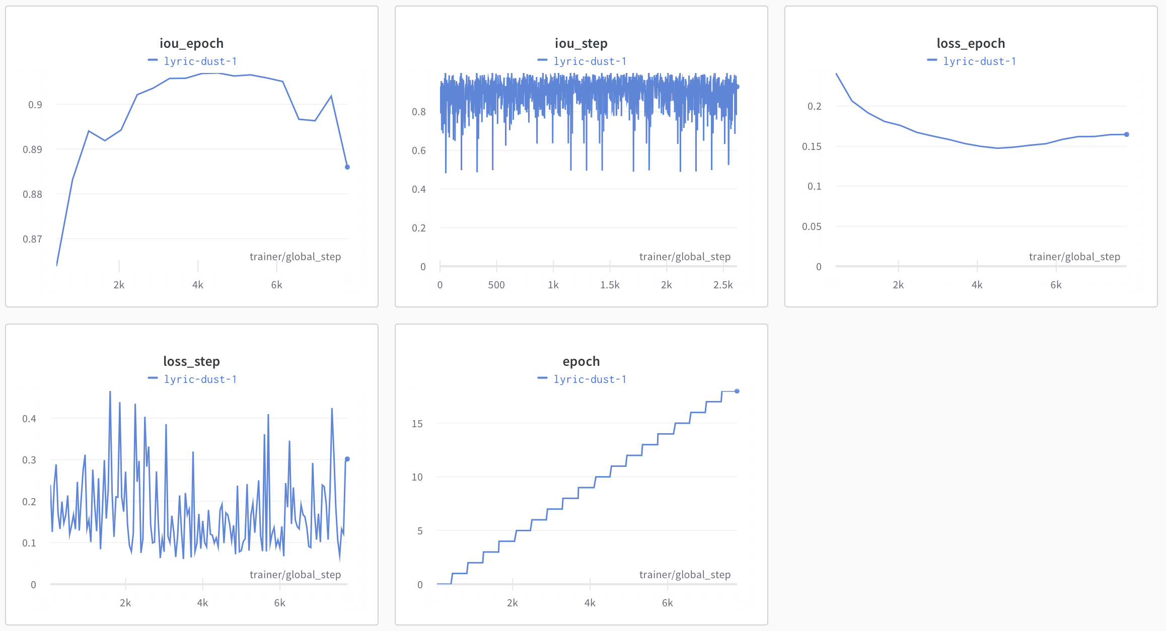
Our plan was to combine the best feature(s) of each set of experiments (backbone, augmentations, etc.) in order to achieve the best result possible. Unfortunately, due to the demand for cloud computing resources, Microsoft Azure denied our group access to the compute resources previously made available freely to us through the Planetary Computer halfway through our experimentation. Azure subsequently declined our offer to pay for compute. We did manage to settle on Google’s Inception-v4 backbone, Adam optimizer, and the ColorJitter augmentation from Albumentations as alterations to the model that demonstrated the highest increased in performance. We were not able to further improve using additional sequences of different augmentations, schedulers apart from CosineAnnealing LR, or cost functions potentially more potent than the vanilla CrossEntropyLoss cost function. All told, however, we did manage to improve performance to achieve an IoU of 0.907 on our validation set, or respectible improvement of 2.25% over the baseline model.